How much information is retained in an average of percentiles?
02 Sep 2021 Tags: Distributed systemsExperienced performance analysts caution against taking averages of percentiles. Gil Tene’s famous 2015 Strange Loop talk, “How NOT to Measure Latency”, features the tip, “You can’t average percentiles. Period.” (at 9:15). Tene offers a brief example using the 100th percentile, the maximum, but does not provide many details. You might think this is enough—simply never average percentiles and you’re safe, right? But as Baron Schwartz points out, the metric pipeline probably averages metrics before you see them, and even displaying metrics as pixels on the screen is a form of averaging. Why is it so bad to average percentiles and how much information does the result retain, if any at all?
Averaging two percentiles
Let’s begin with some examples highlighting the problem. I’m going to use latency distributions, as those are the most common application of percentiles in our industry, but the math is the same for any metric presented as percentiles (or more generally, as quantiles).
As a motivating example, consider a latency metric computed in the following way: Request latencies for a service are collected for one second and the 95th percentile is computed for that sample and stored. The process is repeated every second and the 95th percentiles are reported in a stream to a monitoring system.
For computational simplicity, assume the latencies are distributed continuously and uniformly between 0 and some maximum number of seconds \(m_i\) for sample \(i\). For this distribution, the 95th percentile is simply \(.95 m_i\).
First, consider the case where the rate of traffic has remained the same but response latencies have increased substantially, perhaps because a replicated database on the backend has had one of its replicas crash. The result will be two samples of equal size but with very different P95 percentiles. For two periods we might have:
- Period 1: 1000 samples, \(m_1 = 0.5~\text{s}, \text{P95} = .95 \cdot 0.5 = 0.475~\text{s}\)
- Period 2: 1000 samples, \(m_2 = 1.0~\text{s}, \text{P95} = .95 \cdot 1.0 = 0.950~\text{s}\)
If we simply average these two percentiles, we get .712 s. What is the actual P95? To compute this, we need to compute the latency that bounds 95% of the values in the combined sample. The combined sample has 2,000 values and 95% of that is 1,900.
All 1,000 values in Period 1 are less than or equal to 0.5 s, as well as half the values in Period 2, for a total of 1,500 values. To compute P95, we must bound the 400 remaining values. Given that Period 2 is distributed uniformly, the 400 smallest values greater than 0.5 s are bounded above by 0.900 s, which is the actual P95 for the combined sample. Comparing these statistics:
| Period | Sample size | P95 (s) |
|---|---|---|
| P1 | 1,000 | 0.475 |
| (P951 + P952)/2 | (Not a sample) | 0.712 |
| P1 and P2 combined | 2,000 | 0.900 |
| P2 | 1,000 | 0.950 |
Simply averaging the two percentiles produces an estimate considerably lower than the correct one. Our latency is much worse than suggested by the simple average of the original percentiles. On the other hand, both values, the average and the actual percentile of the combined samples, lie between the two original values. We will see later in this post that this is generally true.
Varying the distributions
The above example used two samples that differed in distribution but were the same size. Sample size also affects the outcome. We can achieve the effect of varying the sample sizes by varying their weight. The following figure and table show how the P95 values vary with the weight of our two distributions:
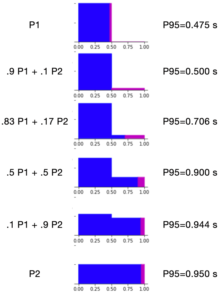
Density plots of six distributions, with their top 5% region highlighted in magenta
| Distribution | 95th percentile |
|---|---|
| 100% 0–0.5 | 0.475 |
| 90% 0–0.5 + 10% 0–1.0 blend | 0.500 |
| 83% 0–0.5 + 17% 0–1.0 blend | 0.706 |
| Naive average (P951 + P952)/2 | 0.712 |
| 50% 0–0.5 + 50% 0–1.0 blend | 0.900 |
| 10% 0–0.5 + 90% 0–1.0 blend | 0.944 |
| 100% 0–1.0 | 0.950 |
As the proportion of the lower-latency distribution decreases from 100% to 0%, the P95 for the combined sample increases from the P95 of the lower-latency distribution up to that of the higher-latency. The naive average of the original P95s happens to correspond most closely to an 83% / 17% weighting of the two distributions. Once again, the P95 values for all blends fall between those of the two original distributions.
The total percentile always lies inside the range of constituent percentiles
In the examples so far, the percentile of the combined samples lay between the percentiles for the two constituent samples. How general is this result? Does it apply beyond the simple uniform distributions used above, to actual latency distributions, which are positively skewed, multimodal, and often have no upper bound? Furthermore, does this result apply to averages over more than two percentiles?
Yes, the percentile for the combination of several samples will always lie between the smallest and largest percentile values for the individual samples, for any underlying distributions and combination of sample sizes. This section will show a simple proof of that result.
This proof applies to the continuous case: Specifically, we require that we can select a subset of each sample that exactly matches an arbitrary proportion \( 0 \le p \le 1 \). No finite sample can satisfy this requirement but sufficiently large samples can approximate it. The phrase “sufficiently large” is vague but the samples typically used in performance analysis of distributed systems, containing hundreds of items or more, meet this requirement. In a future post, I will consider the case of small samples, for which the combined percentile can in fact be outside the range of the percentiles of the constituent samples.
An older post describes the basics of percentiles and the notation that I will use in this section.
Assume we have a set of \(N\) latency samples \(S_i\), each of size \(B_i\), with density \(LD_i(x)\), cumulative distribution \(LC_i(x)\), and percentile function \(LP_i(p)\). For simplicity, we can assume that the distributions \(LD_i(x)\) are nonzero everywhere \(0 < x\) (if this assumption is not met, there are technical solutions that will not change the main results—see Appendix). Under this assumption, the cumulative distributions \(LC_i(x)\) will be strictly monotonic on x, and their inverses, the percentile functions \(LP_i(p) = LC_i(x)^{-1}\), are well-defined.
Consider the \(p\)th percentiles of these samples, \(LP_i(p)\), and let \(LP_1(p)\) be the smallest and \(LP_n(p)\) the largest. Begin with the lower bound. We want to show that the percentile for the combination of all the samples, \(LP_*(p)\), is greater than or equal to \(LP_1\).
Presenting the calculation as a structured derivation:
| \( \bullet \) | \( LP_1(p) \) | \( \le \) | \( LP_i(p) \quad \forall i : 2 \le i \le n \) |
| \( \equiv \) | \( \{ LC_i \text{ is monotonic} \} \) | ||
| \( LC_i(LP_1(p)) \) | \( \le \) | \( LC_i(LP_i(p)) \quad \forall i : 2 \le i \le n \) | |
| \( \equiv \) | \( \{ \text{LHS: let } p_i = LC_i(LP_1(p)) \text{; RHS: } LC_i \text{ and } LP_i \text{ are inverses} \} \) | ||
| \( p_i \) | \( \le \) | \( p \quad \forall i : 2 \le i \le n \) | |
| \( \equiv \) | \( \{ \text{Multiply by positive } B_i \} \) | ||
| \( p_i B_i \) | \( \le \) | \( p B_i \quad \forall i : 2 \le i \le n \) | |
| \( \equiv \) | \( \{ \text{Summing over}\: 2 \le i \le n \} \) | ||
| \( \sum_{i=2}^n p_i B_i \) | \( \le \) | \( p \sum_{i=2}^n B_i \) | |
| \( \equiv \) | \( \{ \text{Adding}\: p B_1 \} \) | ||
| \( p B_1 + \sum_{i=2}^n p_i B_i \) | \( \le \) | \( p B_1 + p \sum_{i=2}^n B_i \) | |
| \( \equiv \) | \( \{ \text{Combine RHS} \} \) | ||
| \( p B_1 + \sum_{i=2}^n p_i B_i \) | \( \le \) | \( p \sum_{i=1}^n B_i \) | |
| \( \equiv \) | \( \{ \text{Divide by positive value } \sum_{i=1}^n B_i\} \) | ||
| \( \frac{p B_1 + \sum_{i=2}^n p_i B_i}{\sum_{i=1}^n B_i} \) | \( \le \) | \( p \) | |
| \( \equiv \) | \( \{ LP_* \text{ is monotonic} \} \) | ||
| \( LP_*(\frac{p B_1 + \sum_{i=2}^n p_i B_i}{\sum_{i=1}^n B_i}) \) | \( \le \) | \( LP_*(p) \) | |
| \( \equiv \) | \( \{ \text{Show equivalence to } LP_1(p) \} \) | ||
| \( \bullet \quad LP_*(\frac{p B_1 + \sum_{i=2}^n p_i B_i}{\sum_{i=1}^n B_i}) \) | |||
| \( \equiv \quad \{ \frac{p B_1 + \sum_{i=2}^n p_i B_i}{\sum_{i=1}^n B_i} \text{ is exactly the proportion of the combined sample } \le LP_1(p) \} \) | |||
| \( \quad \; LP_1(p) \) | |||
| \( \cdots \) | \( LP_1(p) \) | \( \le \) | \( LP_*(p) \) |
| \( \Box \) | |||
Analogous logic proves the upper bound, \(LP_*(p) \le LP_n(p)\). Combining these, we have proven:
Combined Percentile Theorem (Continuous case): For a collection of \(n\) samples, each with an arbitrary distribution and sample size and each of which can be subdivided to arbitrary precision,
\[ LP_1(p) \le LP_*(p) \le LP_n(p) \]
where \(LP_1(p)\) and \(LP_n(p)\) are the smallest and largest percentiles in the collection, respectively.
Combining this theorem with the widely-known result that an average lies within the range of its constituent values, we get:
Corollary (Continuous case): The average of the \(p\)-percentiles for a collection of infinitely subdividable samples will be at most \(LP_n(p) - LP_1(p)\) from the \(p\)-percentile of the combined samples, \(LP_*(p)\).
Conclusion
The average of the percentiles for a collection of samples is not the same as the percentile for the combined samples but its deviation from the combined percentile is bounded. So long as the the samples are large and their percentiles are near one another, their average will be close to the combined percentile whereas if the percentiles are widely-spaced, their average could be distant from it.
We have also seen that when reasoning about combined percentiles, we have to consider both the distributions they represent and the sizes of the individual samples.
In the next post, I’ll consider the implications of these results for some typical uses of percentiles in dashboards.
Appendix—When the density function has regions at zero
In this appendix, I briefly discuss the case where a sample’s distribution has a region where its density function is 0.
Wherever \(LD_i(x)\) has a zero region, \(LC_i(x)\) will be a flat line seqment. For the proportion \(q = LC_i(x)\), we could define the percentile \(LP_i(q)\) to be any \(x\) within that region. Define \(LP_i(q)\) to be the smallest such \(x\). With this definition, we retain the key identity
\[ LC_i(LP_i(p)) = p \]
required in the above proof.
Under these revised definitions, \(LC_i\) is weakly monotonic and \(LP_i\) remains strongly monotonic. The above proof only requires that both be at least weakly monotonic.
Consequently, all transformations in the proof continue to apply and so the proof holds.