The basics of latency percentiles

Designers of distributed systems obsess over service latency. They forecast latencies of proposed designs, stress-test the latencies of systems under development, equalize latencies of replicated services by load balancing, monitor latencies of production systems using instrumentation, and commit to latency targets in service level objectives and agreements.

The most commonly-used representation of latency in these scenarios is percentiles. Percentiles are deceptively simple, a function from values between 0 and 1 (or equivalently 0% and 100%) to a response time. But the relation between percentiles and the distribution they describe is subtle: Formally, the percentile function is the inverse of the integral of the probability density of the distribution.

The subtlety of this construction makes it easy to miss a step and become confused. Working through the basics in detail, gaining a clear understanding of how percentiles relate to other representations of latency, provides designers with a straightforward approach to reasoning about a fundamental concept in distributed systems design.

Latency distributions

Begin with distributions. The latency distributions of actual services do not conform well to any of the widely-studied distributions presented in statistical texts. Distributions of latencies are:

1. Positively skewed, with a heavy tail on the right
2. Time-varying
3. Multimodal
4. Spiky
5. Bounded below but not above.

There is an interesting analysis to be done, showing these properties as consequences of the underlying mechanisms in our systems. For this article, I will simply note that these properties are widely-observed in the distributions of actual systems, including Gil Tene’s classic rant and Ben Sigelmen’s argument that “performance is a shape”.

Representing latency by a density function

Designers typically envision latency as a density function, with latency the horizontal axis, beginning at zero and unbounded in the positive direction, while the vertical axis is an abstract nonzero probability density.

The density function \(LD(t)\) for latencies has the following properties:

• \(LD(t) = 0, \quad t <= 0\)
• \(0 < LD(t), \quad t > 0\)
• \(\lim_{t\to\infty} LD(t) = 0\quad(LD(t)\) is asymptotic to the horizontal axis)
• \(\int_0^\infty LD(t) \,\mathrm{d}t = 1\quad\) (the area under \(LD(t)\) is 1)

A simplified latency distribution

For purposes of this post, I will need an example distribution. I do not propose this distribution as representing any actual distribution but simply use it to represent some of the complexities of actual latencies. Any description of actual latencies will have to include these complexities at the least.

The example distribution is the mixture of two lognormal distributions:

• 80% a lognormal density for a random variable whose log is a Gaussian with mean 0 and standard deviation 1.0
• 20% a lognormal density for a random variable whose log is a Gaussian with mean 5 and standard deviation 0.5.

The SciPy code for this density function is:

lambda x : .8 * stats.lognorm.pdf(x, 1.0) +
           .2 * stats.lognorm.pdf(x, 0.5, loc=5.0)

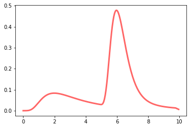
and it has the following density function:

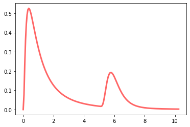
The resulting mixture matches several properties of actual latency distributions:

1. Bounded below by 0
2. Asymmetric, with a long positive tail
3. Multimodal (in this case, bimodal)

The density plot is likely what most designers have in mind when imagining the latency distribution of an actual or prospective service. How is this related to percentiles, the measure typically used to characterize latencies? The process is indirect, comprising several steps, and it’s informative to walk through them in detail.

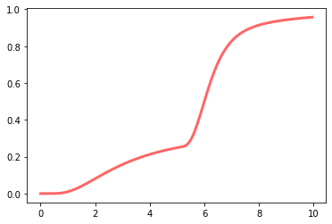
Step 1: Compute the cumulative distribution

The first step is computing the cumulative distribution, \(LC(t)\). Analytically, this is just the integral of the density:

\[ LC(t) = \int_0^t LD(x) \,\mathrm{d}x \]

The cumulative distribution has the same domain as the density, a range of [0, 1), and an important additional property: For actual latency distributions, it is strictly monotonically increasing:

\[ \forall\: t1, t2, t1 < t2 :\: LC(t1) < LC(t2) \]

(Although one can construct distributions whose corresponding cumulative function is monotonic but not strict, these are extremely rare in practice. If one should arise, there are technical solutions to make its cumulative function strictly monotonic.) This property is essential for computing the percentile, as we will see in the next step.

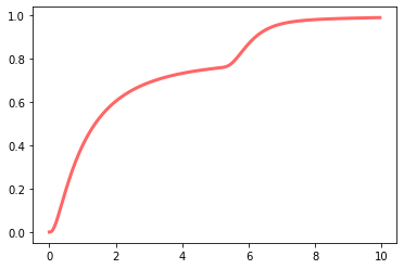
For the sample distribution given above, the cumulative distribution \(LC(t)\) is:

Step 2: Compute the inverse cumulative distribution

The percentile function, \(LP(p)\), is the inverse of the cumulative distribution:

\[ LP(p) = LC(t)^{-1} \]

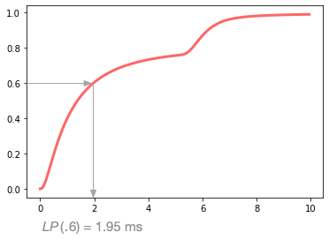
The strict monotonicity of \(LC(t)\) we described above ensures that its inverse is well-defined. The following diagram illustrates how \(LP(.6)\) is computed, drawing a ray from .6 on the range of \(LC(.6)\) until it intersects the function, then dropping to 1.95 ms on the domain:

Heights in \(LP\) are areas under \(LD\)

I think it’s helpful to explicitly show the relationship between the percentile \(LP\) and the density \(LD\). As the inverse of the integral, a height in \(LP\)

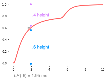
corresponds to an area under \(LD\):

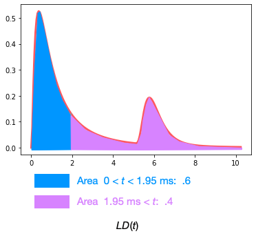
Those shapes are deceptive: I had to run a numeric integration to convince myself that the cyan area is in fact 50% larger than the magenta.

Using the tools: Computing effective percentile \(EP\)

Understanding the detailed construction of \(LP(p)\) helps explain the details of computing effective percentiles. Consider the computation of \(EP(.6, 5)\), the effective percentile corresponding to the slowest response of 5 calls to a service with \(LP(.6) = 1.95\) ms. The effective percentile is \(EP(.6, 5) = .078\). Graphically, the cumulative probability at 1.95 ms is dropped from .600 to .078

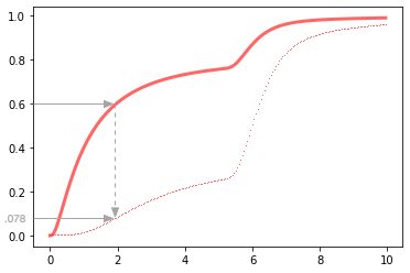
producing an effective cumulative distribution \(EC(t, 5)\) (where 5 is the fanout):

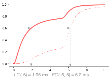
This illustrates how the probability of high latencies has increased due to five calls to the service. Where the original \(LC(1.95~\mathrm{ms}) = .6\), now we have to go up to 6.2 ms to get \(EC(6.2~\mathrm{ms}, 5~\mathrm{calls}) = .6\):

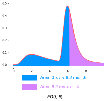
Differentiating the cumulative function from time \(t\) and fanout \(f\) \(EC(t, f)\) over \(t\) gives us the effective density \(ED(t, f)\):

The shape of this density function informs our intuition of the effect of multiple calls to a service: We squeezed the left side of the density, causing the right side to expand. For example, separating the density into regions of .6 and .4 of the total area, we see how the density has shifted right compared to the original density function \(LD(t)\) shown above:

Summary

Latency percentiles are simple but subtle. Understanding their construction from the original density distribution clarifies important concepts such as effective percentiles.